Guide to Text Classification with fastai

With thorough explanation of Classes and Methods from fastai.text

With the advent of Transfer Learning, language models are becoming increasingly popular in text classification and many other problems in Natural Language Processing. Previous approaches to these problems included using word embeddings, which stores only semantic similarity between words. However, embeddings are limited in their understanding of the context and multiple meanings of a word are conflated to a single representation. 

Language models have shown to be more capable of understanding the context and terminologies which are specific to the text of the input data. Thus, they are proficient in generating text, and they can be used to improve the accuracy of text classifier models.

In this post, you will learn the different classes and methods required to build a text classification model using Transfer Learning on the popular fastai library.

For our example we will be using a dataset containing 1.6 million tweets extracted from the Twitter API. This data has been annotated for sentiment analysis in the following manner:

0=negative

2=neutral

4=positive

We will begin by processing the input text data into vectors which can be interpreted by the machines, then we will create a language model. This model will learn the context which is specific to the input text data, and it will predict the next word in a sentence. Using the representations used by the language model, we will create a classification model, which predicts the sentiment score of a given tweet.

Below is a flowchart containing all the classes and methods required for the creation of a text classification model :

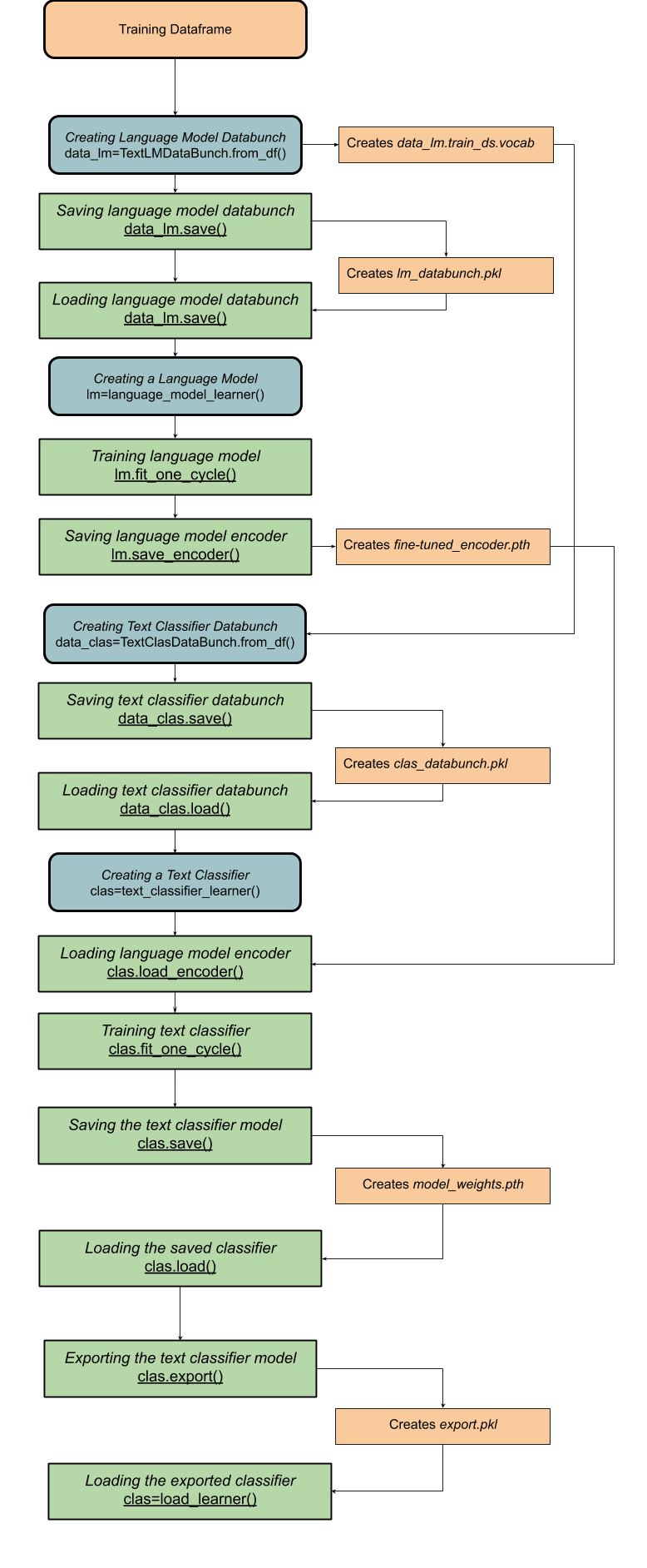
The process has been broken down into the following stages:

1. Importing the data

2. Creating Datasets for Language Model

3. Creating the Language Model

4. Creating the Classifier Model

5. Saving and Loading Models

6. Testing the Classifier Model

Importing the Data

We will be working on Google Colabatory, which is based on Jupyter, running in a browser, and the only requirement is a Google Drive account.

The Twitter dataset is available as a .csv file which can be download from Kaggle: https://www.kaggle.com/kazanova/sentiment140

Go ahead and upload the unzipped .csv file to Google Drive, and rename the file to “training.csv”.

We will be importing the following functions and packages for this project:

import numpy as np  
import pandas as pd
from pathlib import Path
from fastai.text import *

We begin by mounting the Google Drive in our notebook:

from google.colab import drivedrive.mount(‘/content/gdrive’)

The output of the command will look like this:

Copy and paste the authorization code in the provided cell.

Then we read in the data, and provide names to the columns:

path=Path(‘/content/gdrive/My Drive’)

df= pd.read_csv(path/”training.csv”, encoding=’latin-1')

df.columns[‘Sentiment_Score’,’ID’,’Time’,’Query_Status’,’Account_Name’,’Tweet’]

From the dataframe, we will be creating a training dataset and a validation dataset by splitting it into a 80:20 ratio.

df = df.iloc[np.random.permutation(len(df))]

cut1 = int(0.8 * len(df)) + 1

df_train, df_valid = df[:cut1], df[cut1:]

Creating Datasets for Language Model

The input text data is broken down into individual words, and then each word is represented by a vector. The TextLMDataBunch method creates a language model databunch object which stores the vector representation of all unique words as tokens. Now, the computer can use this object to create a language model.

data_lm = TextLMDataBunch.from_df(path=path, 

                                  train_df=df_train,

                                  valid_df=df_valid,

                                  label_cols=’Sentiment_Score',

                                  text_cols=’Tweet’)

Once the databunch object is created, it can be saved using 

data_lm.save(path,'filename.pkl')

which saves it as a pickle file(.pkl)

 and then loaded on again simply using

data_lm.load(path, 'filename.pkl')

Creating the Language Model

A language model is created using the language_model_learner command which creates a language model based on the previously created databunch object . The language model can be trained to understanding the language better and the context of the input text data. We create the model using a recurrent neural network(RNN), and we will be using the AWD_LSTM architecture:

lm = language_model_learner(data_lm, AWD_LSTM, drop_mult=0.3)

Language model encoder, encodes the input text it into a vector representation, and the decoder uses the encoded vector to predict the next word. In text classification, we do not want to predict the next word of a sentence, so we remove the decoder, removing the layers which predict the next word and replace them with layers which predict the sentiment score of a tweet.

lm.save_encoder(path/'filename.pth')

only saves the encoder of the language model as a Windows Pathname Document(.pth)

Creating the Classifier Model

Now we will be using the TextClasDataBunch method to create a classifier databunch object, which can later be used to train the classifier model. 

The group of tokens which was created for the language model databunch object are stored in a dictionary, known as the vocab, which stores the tokenised version of each word. We want to use the same vocabulary for the classifier model, to implement the fine-tuned language model later. Thus, we extract the location ID of each token from the language model databunch object and assign our classifier databunch to use these ID tokens by passing in vocab=data_lm.train_ds.vocab in our command :

data_clas=TextClasDataBunch.from_df(path=path,

                                    train_df=df_train,

                                    valid_df=df_valid,

                                    vocab=data_lm.train_ds.vocab,

                                    label_cols=’Sentiment_Score’,

                                    text_cols=’Tweet’)

Using text_classifier learner, we create the model which can predict the sentiment score of the tweet:

clas = text_classifier_learner(data_clas,AWD_LSTM,drop_mult=0.3)

Then we load the encoder of the language model using

clas.load_encoder(path/’filename.pth’)

We can create the final layers which predict the classifier tag, by training the model using

clas.fit_one_cycle(number of cycles, learning rate)

The optimal learning rate can be found using 

clas.lr_find()

clas.recorder.plot(suggestion=True)

Saving and Loading Models

The language and classifier models can be saved and loaded in 2 ways:

1. Learner.save(): This method only saves the weights of the model, as a Windows Pathname Document(.pth). This method is used to save the model in its intermediate stage, and then loaded to resume the training of the model.

learner.save(‘filename.pth’)

Once the model is instantiated(i.e. defining the learner object and its classes), we can load the weights of the model using

learner.load(‘filename.pth’)

2. Learner.export(): This method saves all the objects required by the language model: the transforms, classes, normalization of data, model and its weights. It saves as a Pickle file(.pkl) with the name (‘export.pkl’). This method is used once the model has completed its training, and it is prepared to be deployed.

learner.export(path)

which saves the model into a Pickle file with the name export.pkl. 

The model can then be called upon anytime, without the requirement of any instantiation, using

load_learner(path)

Testing the Classifier Model

Once the model is created, now you can test the model using the following methods:

1. Learner.predict(data) can be used to predict the class and probability of a particular piece of data, which is entered.

2. Learner.get_preds(ds_type=DatasetType.Test) can be used to predict the class and probability of each item in a specified dataset.

Also posted on Medium

Author: Chandramoulli Singh